Representing Graphs
Adjacency Matrix
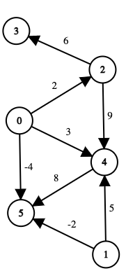
In an adjacency matrix m, the cell m[i][j] represents the edge weight from node i to node j.
[[0,0,2,0,3,-4],
[0,0,0,0,5,-2],
[0,0,0,6,9,0],
[0,0,0,0,0,0],
[0,0,0,0,0,8],
[0,0,0,0,0,0]]
The matrix represents the graph in the picture above.
| Pros | Cons |
|---|---|
| Space efficient for representing dense graphs | Requires O(V2) space |
| Edge weight lookup is O(1) | Iterating over all edges takes O(V2 time |
| Easy to understand |
Adjacency List
An adjacency list represents a graph as a map from nodes to list of edges. The first value in the tuple represents the to node and the second value represents the weight. It is most commonly used in solving graph problems.
0 -> [(2,2),(4,3),(5,-4)]
1 -> [(4,5),(5,-2)]
2 -> [(3,6),(4,9)]
3 -> []
4 -> [(5,8)]
5 -> []
| Pros | Cons |
|---|---|
| Space efficient for representing sparse graphs | Less space efficient for denser graphs |
| Iterating over all edges is efficient | Edge weight lookup is O(E) |
| Slightly more difficult to understand |
Edge List
An edge list is an unordered list of edges. The triplet (u,v,w) means the cost from node u to node v is weight w. It is seldom used because of its lack of structure.
[(2,3,6),
(2,4,9),
(0,2,2),
(0,4,3),
(0,5,-4),
(4,5,8),
(1,4,5),
(1,5,-2)]
| Pros | Cons |
|---|---|
| Space efficient for representing sparse graphs | Less space efficient for denser graphs |
| Iterating over all edges is efficient | Edge weight lookup is O(E) |
| Very simple structure |